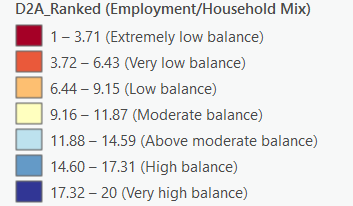
The employment–household mix indicator measures the balance between employment opportunities and residential households within a municipality. The scores represent municipal averages of the U.S. Environmental Protection Agency’s ranked Employment–Household Mix (D2A_Ranked) variable, which ranges from 1 to 20. Higher scores indicate a more balanced relationship between jobs and housing, while lower scores reflect greater separation between residential areas and places of employment.

Employment–household mix is one of the three land-use components incorporated into the National Walkability Index. Communities where employment opportunities and housing are more closely balanced generally support shorter trips, greater accessibility, and increased opportunities for walking, bicycling, and transit use. By contrast, communities dominated by either residential development or employment uses often require longer commuting distances and greater dependence on automobiles.

Unlike the complete National Walkability Index, this measure evaluates only the relationship between jobs and households. It does not account for street connectivity, transit accessibility, sidewalks, or pedestrian infrastructure, all of which also influence walkability.

Classification Categories

• Very High Employment–Household Mix (17.32–20.00): Municipalities with an exceptionally balanced relationship between employment opportunities and residential households. Jobs and housing are closely integrated, supporting shorter commutes and greater opportunities for active transportation.
• High Employment–Household Mix (14.60–17.31): Municipalities where employment and residential development are well balanced. Residents generally have convenient access to employment within or near the municipality.
• Above Average Employment–Household Mix (11.88–14.59): Municipalities with relatively strong job-housing balance. Employment centers and residential neighborhoods are reasonably well integrated, reducing the need for long-distance commuting.
• Moderate Employment–Household Mix (9.16–11.87): Municipalities with a moderate balance between jobs and households. Some residents work locally, while many commute to surrounding communities.
• Below Average Employment–Household Mix (6.44–9.15): Municipalities where either employment or housing substantially outweighs the other. Commuting patterns become increasingly regional rather than local.
• Low Employment–Household Mix (3.72–6.43): Municipalities with significant imbalance between residential development and employment opportunities. Residents typically rely heavily on neighboring municipalities for work or housing.
• Very Low Employment–Household Mix (1.00–3.71): Municipalities exhibiting extreme job-housing imbalance. These communities often function almost entirely as residential suburbs, employment centers, or specialized land uses with very limited local balance.

Planning Implications

A balanced relationship between employment and housing is widely recognized as an important component of sustainable urban development. Communities that provide both employment opportunities and residential neighborhoods within close proximity reduce commuting distances while increasing transportation choices.

Higher employment–household mix generally supports:

• Shorter average commuting distances.
• Greater opportunities for walking, bicycling, and transit use.
• Reduced automobile dependency.
• More resilient local economies.
• Increased support for mixed-use and infill development.
• Greater efficiency in transportation and public infrastructure investments.

Communities with lower employment–household mix may improve local accessibility through mixed-use zoning, encouraging residential development near employment centers, attracting employers to residential communities, or promoting redevelopment that better balances jobs and housing over time.

However, employment–household balance alone does not ensure walkability. Safe pedestrian infrastructure, connected street networks, transit accessibility, and nearby daily destinations remain essential components of a walkable community.

Understanding Municipal Employment–Household Mix

Municipal employment–household mix scores provide a standardized method for comparing one dimension of land-use balance across communities. The EPA calculates this indicator using the relationship between employment and households within Census block groups before ranking each location on a national scale. Municipal scores represent averages of those ranked values.

Higher scores generally indicate municipalities where employment opportunities and housing are more evenly distributed, reducing the separation between where people live and where they work. Lower scores often reflect communities dominated by either residential development or employment uses, increasing regional commuting demands.

For example, municipalities such as Orlando (12.34), Boise (12.10), Raleigh (12.02), Portland (11.90), Greensboro (11.89), Austin (11.53), and Atlanta (11.30) demonstrate relatively balanced employment–household relationships within their municipal boundaries.

Conversely, municipalities such as Detroit (6.51), Las Vegas (8.44), Chicago (8.34), Philadelphia (8.36), Dallas (8.84), Baltimore (8.81), and New Orleans (8.30) receive lower employment–household mix scores despite serving as major regional employment centers. These results illustrate that municipal averages are influenced by municipal boundaries, suburban growth, and regional commuting patterns rather than simply total employment.

Because municipal averages combine neighborhoods with varying land-use characteristics, they should be interpreted as broad indicators rather than neighborhood-level measurements.

Geographic Patterns in Municipal Employment–Household Mix

Employment–household mix varies considerably across the United States due to differences in metropolitan structure, economic specialization, and development patterns.

• Major Metropolitan Areas: Large cities often exhibit moderate employment–household balance because employment is distributed across multiple municipalities rather than concentrated entirely within the central city.
• Mixed-Use Municipalities: Communities that combine residential neighborhoods with office districts, commercial corridors, institutional campuses, and industrial areas frequently receive higher scores because jobs and housing are more evenly balanced.
• Suburban Residential Communities: Many suburban municipalities receive lower scores when residential growth substantially exceeds local employment opportunities, resulting in greater outbound commuting.
• Employment Centers: Municipalities dominated by airports, industrial parks, military installations, or major office districts may also receive lower scores because employment substantially exceeds residential development.
• Small Cities and Rural Communities: Scores vary depending on whether local employment opportunities adequately serve the resident population or whether the municipality functions primarily as a residential community.

These geographic patterns illustrate that employment–household mix reflects both local land-use planning decisions and broader metropolitan economic relationships.

Relationship to Walkability

Employment–household balance is a fundamental component of walkability because it directly influences travel demand and commuting patterns. Communities where housing and employment are located closer together reduce average trip lengths and increase opportunities for walking, bicycling, and public transit.

Research by Cervero and Kockelman (1997) identified land-use diversity as one of the “3Ds” (Density, Diversity, and Design) that shape travel behavior. Ewing and Cervero (2010) later confirmed through a meta-analysis that balanced land-use patterns are consistently associated with reduced vehicle travel and increased walking and transit use. Frank et al. (2006) similarly demonstrated that neighborhoods combining diverse land uses with connected transportation networks support healthier travel behavior and greater physical activity.

Although employment–household mix captures an important aspect of accessibility, it should always be interpreted alongside street connectivity, transit accessibility, and pedestrian infrastructure to provide a comprehensive assessment of municipal walkability.

Overall Pattern

Municipal employment–household mix highlights how effectively communities balance places to live with places to work. Municipalities with higher scores generally provide better opportunities for residents to access employment without lengthy commutes, supporting more efficient transportation systems and greater opportunities for active travel. Lower scores often reflect specialized land-use patterns or regional commuting relationships rather than poor economic performance.

Consequently, employment–household mix should be interpreted as a measure of job-housing balance rather than economic strength. The indicator evaluates how well employment opportunities and residential development are integrated within the built environment, making it an important component of understanding accessibility and walkability across American municipalities.

References

- Cervero, R., & Kockelman, K. (1997). Travel Demand and the 3Ds: Density, Diversity, and Design.Transportation Research Part D: Transport and Environment, 2(3), 199–219.
- Duany, A., Plater-Zyberk, E., & Speck, J. (2010). Suburban Nation: The Rise of Sprawl and the Decline of the American Dream(10th Anniversary). North Point Press.
- Ewing, R., & Cervero, R. (2010). Travel and the Built Environment: A Meta-Analysis.Journal of the American Planning Association, 76(3), 265–294.
- Frank, L. D., Sallis, J. F., Conway, T. L., Chapman, J. E., Saelens, B. E., & Bachman, W. (2006). Many Pathways from Land Use to Health: Associations between Neighborhood Walkability and Active Transportation, Body Mass Index, and Air Quality.Journal of the American Planning Association, 72(1), 75–87.
- North End, Boston. (2026). In Wikipedia. https://en.wikipedia.org/w/index.php?title=North_End,_Boston&oldid=1358627339
- O’Boyle, J. (November 3). Tips for Visiting Greenwich Village, NYC. The Empty Nest Explorers. https://www.theemptynestexplorers.com/blog/tips-for-visiting-greenwich-village-nyc
- S. Environmental Protection Agency. (2021b). Smart Location Database (SLD) 3.0: Technical Documentation and User Guide. U.S. Environmental Protection Agency. https://www.epa.gov/smartgrowth/smart-location-mapping#SLD
- U.S. Environmental Protection Agency. (2021a). National Walkability Index: Methodology and User Guide. U.S. Environmental Protection Agency (EPA). https://www.epa.gov/smartgrowth/smart-location-mapping#walkability